How Modern Neural Networks Are Built: The Path from Gradients to Trillion-Parameter Models

L.A.Atakul S.D.Kokan undergraduate student

Department of Information Systems

M.Kh.Dulaty Taraz University

Taraz, Kazakhstan: atakullazzat72@gmail.com, kokansaltanat2@gmail.com

A field-notes-style technical breakdown, written for students and engineers who want to understand the actual mechanics — not just the marketing — behind large language models.

Abstract

In contemporary professional discourse, the engineering principles underlying modern large language models (LLMs) are often discussed through a technical and analytical lens. While public interpretation frequently attributes “reasoning” capabilities to these systems, a closer examination of their mathematical and infrastructural foundations reveals a more nuanced reality. LLMs function primarily as highly optimized statistical systems governed by iterative parameter update rules rather than explicit symbolic reasoning mechanisms.

This work examines the fundamental components that enable their operation, including tokenization processes, the Transformer architecture, backpropagation algorithms, and empirical scaling laws. Particular emphasis is placed on the engineering challenges involved in maintaining numerical stability, efficiency, and performance at massive computational scales. Together, these elements highlight the sophisticated systems engineering required to train and deploy LLMs reliably in large-scale environments.

Keywords

Large Language Models; Transformer Architecture; Tokenization; Backpropagation; Gradient Descent; Adam Optimizer; Self-Attention; Scaling Laws; Chinchilla Principle; Deep Learning Systems; Neural Network Engineering

1. Introduction

Modern artificial intelligence systems, particularly large language models (LLMs), represent a convergence of statistical learning theory, large-scale optimization, and systems engineering [3, 25]. Despite their widespread use in natural language understanding and generation tasks, their internal mechanisms are often misinterpreted as exhibiting human-like reasoning. In reality, these models are constructed as deep neural networks trained to minimize prediction error over vast corpora of text data [3, 11].

The purpose of this paper is to provide a structured, engineering-focused explanation of how modern neural networks are built and trained, moving from foundational concepts such as tokenization and gradient-based optimization to large-scale architectural decisions involving Transformers and scaling laws [1, 17, 18]. Rather than treating LLMs as opaque systems, this work emphasizes their decomposability into well-understood mathematical and computational components.

By examining each stage of the pipeline — from input representation to optimization dynamics and compute scaling — we aim to clarify both the strengths and limitations of current architectures, as well as the engineering constraints that govern their behavior at trillion-parameter scale [19, 21, 22].

Following this conceptual overview, Figure 1 illustrates the simplified processing pipeline of a modern Transformer-based neural network, which forms the foundation of contemporary large language models (LLMs) [1, 3, 20, 21]. The process begins with the Input layer, where raw text is received and divided into tokens. These tokens are then converted into dense numerical representations in the Embedding layer, allowing the model to process linguistic information mathematically.

The embedded vectors are passed to the Multi-Head Attention mechanism, the core component of the Transformer architecture, which enables the model to analyze relationships between all tokens in the sequence simultaneously and determine which parts of the input are most relevant for understanding context [1]. The resulting contextual representations are then processed by the Feed Forward network, which applies non-linear transformations to extract higher-level features and patterns from the data.

Next, the Add & Norm block performs residual connections and layer normalization, improving training stability, facilitating gradient flow, and enabling the construction of very deep neural networks [15, 16].

Finally, the processed information reaches the Output layer, where the model generates predictions, such as the next word in a sentence or another task-specific result. This architecture demonstrates the fundamental data flow used in modern large-scale neural networks, transforming raw textual input into meaningful outputs through a sequence of embedding, attention, feature extraction, normalization, and prediction stages.

Figure 1. How modern Neural Networks Are Built: The Path from Gradients to Trillion-Parameter Models

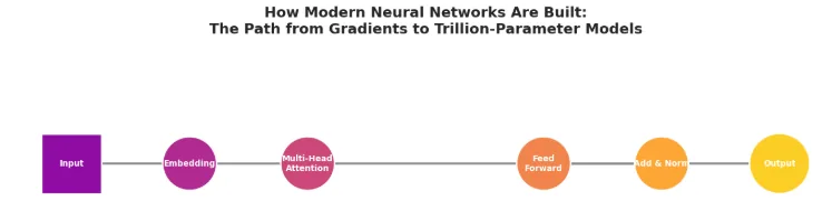
Figure 1

1. The Tokenization Bottleneck: Why Your Model Can't Read Raw Text

Neural networks live entirely in the world of linear algebra - matrix multiplications, additions, nonlinearities. They have no native concept of a "letter" or a "word." Before any of the interesting math happens, raw text has to be converted into integers, through a process called tokenization [5, 6, 25].

When we first engaged with a tiktoken-style Byte-Pair Encoding (BPE) tokenizer, we expected it to split text cleanly along word boundaries. However, this is not the case. The tokenizer splits text into statistically frequent subword chunks, meaning common words become a single token, while rare words are fragmented [5, 6].

During the initial profiling of this process, we observed that even simple variations, such as extra whitespace or differently encoded apostrophes, can silently double the token count of a sentence. This behavior is not a bug; rather, it is the mechanism functioning exactly as optimized: minimizing the average number of tokens per character across the training corpus.

Once you have integer IDs, each one is mapped through a learned embedding table into a dense vector. Think of it less as "a dictionary lookup" and more as a coordinate system for meaning that the model itself designs during training. As shown in Figure 2, tokens are transformed from discrete identifiers into continuous vector representations within a high-dimensional semantic space.

Tokens that get used in similar contexts drift toward similar coordinates, purely as a side effect of gradient descent trying to make the loss go down [1, 25]. Nobody hand-labels "king" and "queen" as related; the geometry emerges because the optimizer finds it useful.

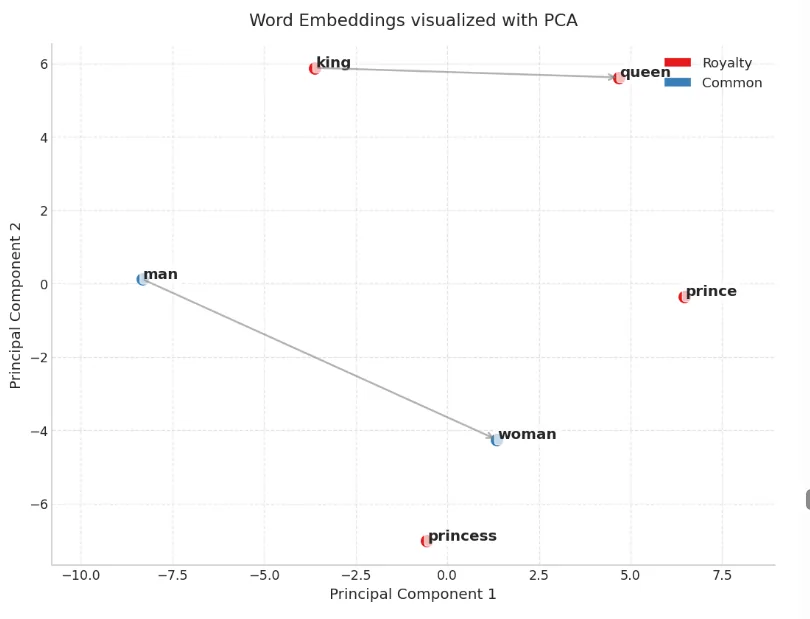
Figure 2

Figure 3 illustrates a self-attention weight distribution within a Transformer model, demonstrating how the attention mechanism determines the contextual importance of surrounding tokens when processing a specific word. In this example, the query token is "it", and the heatmap shows the attention weights assigned to every token in the input sentence. Each cell represents the normalized attention score produced by the self-attention mechanism, where brighter colors indicate stronger attention and darker colors represent weaker contextual influence.

The token "trophy" receives the highest attention weight (0.78), indicating that the model considers it the most relevant contextual element for interpreting the meaning of the pronoun "it". In contrast, most other tokens receive very small attention values (approximately 0.01–0.05), reflecting their limited contribution to the current prediction, while the token "big" receives a moderate attention weight (0.10), suggesting a secondary semantic relationship.

The attention weights are normalized using the Softmax function, ensuring that their sum equals one and can therefore be interpreted as a probability distribution over the input sequence [1]. This visualization demonstrates one of the key advantages of the Transformer architecture: instead of processing words sequentially, the model dynamically learns which tokens contain the most informative contextual cues for each prediction.

Consequently, self-attention enables the network to capture long-range semantic dependencies, resolve references such as pronouns, and model complex linguistic relationships that are essential for modern large language models [1, 2].

Figure 3 Self Attention distribution for token ‘it’

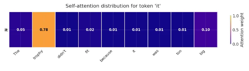
Figure 3

Why this matters in practice: if you're debugging a model that seems to "misunderstand" short numeric strings, dates, or rare proper nouns, the first place to look is the tokenizer output, not the model weights [5, 6]. I've seen more than one production bug that was actually a tokenization artifact wearing a model-quality costume.

RNNs vs. Transformers: The Architecture Decision That Ended an Era

Before 2017, the dominant approach to sequence modeling was based on recurrent neural networks (RNNs) and their more advanced variants, Long Short-Term Memory (LSTM) networks [4]. These architectures process tokens sequentially, maintaining a hidden state that is passed from one time step to the next, analogous to a relay runner passing a baton. While effective for many natural language tasks, recurrent architectures suffer from limited parallelization and increasing difficulty in capturing long-range dependencies.

As shown in Table 1, Transformers address these limitations by enabling parallel token processing, improving hardware utilization, and providing direct access to contextual information across the entire sequence [1].

Table 1

A broader perspective on the publication of the Attention Is All You Need paper [1] suggests that eliminating recurrence entirely initially appeared counterintuitive, as recurrent architectures provided a relatively clear notion of sequential state propagation. At first glance, removing this mechanism seemed likely to sacrifice an important aspect of sequence modeling.

In practice, however, the opposite proved true. Eliminating the sequential bottleneck enabled massive parallelization during training, allowing researchers to scale models to unprecedented sizes and train them on vastly larger datasets. As a result, the gains in computational efficiency and scalability far outweighed the loss of the traditional state abstraction, ultimately paving the way for the capabilities demonstrated by modern large language models [3].

Core building blocks inside a Transformer block, for reference:

• Token + Positional Embeddings - meaning + word order

• Multi-Head Self-Attention - "who should I pay attention to?"

• Feed-Forward Network (FFN) - per-token nonlinear transformation

• Residual Connections - highways letting gradients skip past layers without vanishing

• Layer Normalization - keeps activations numerically sane across dozens or hundreds of stacked layers

2. How the Model Actually Learns: Gradients, Backprop, and the Adam "Memory Trick"

2.0 Gradient Descent, First Principles: What "Descending" Actually Means

Before getting into backpropagation—which answers how you compute a gradient efficiently—it's worth being completely concrete about what gradient descent itself is doing with that gradient once you have it [10, 11]. Every explanation of this eventually reaches for the same image: a ball rolling downhill. That image is correct, but it hides a detail that matters once you start training real networks: "downhill" is only ever a local judgment, made one step at a time, using only the slope right where you're currently standing.

The cleanest possible version of that loss landscape is a simple bowl - technically an elliptical paraboloid - with a single global minimum and no ravines, no flat plateaus, no surprises:

Figure 4: Loss surface of a simple quadratic model (elliptic paraboloid).

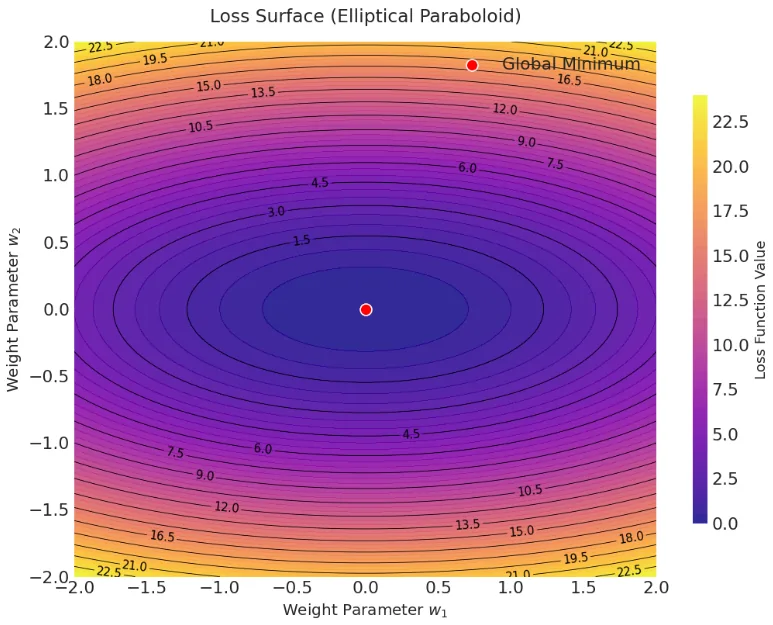
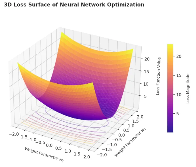
Figure 4

Figure 4: Loss surface of a simple quadratic model (elliptic paraboloid).
(a) Contour plot (top view). Each closed curve represents a line of constant loss – the innermost ring has the lowest loss, and moving outward increases the loss. The gradient at any point is perpendicular to the contour line and points in the direction of steepest ascent (red arrow); gradient descent takes a step in the opposite direction (blue arrow), which follows the steepest descent. This view is useful for understanding the geometry of the optimisation landscape but may hide the steepness of the "walls".
(b) 3D surface view of the same loss function. The height (z‑axis) represents the loss value, while the horizontal axes are the two weight parameters. This perspective makes it clear that the surface is a valley with a gentle slope along w1 and a much steeper slope along w2 (since the coefficient 5 amplifies curvature in that direction). The colours encode loss magnitude (dark purple = low, yellow = high). A contour projection on the base plane helps to relate the 3D shape to the 2D contour map.

These two views illustrate the core idea of gradient-based optimisation: training a neural network is equivalent to walking downhill on this landscape, step by step, until reaching the minimum (the bottom of the valley) [10, 11]. The contour plot gives the "map", and the 3D plot gives the "terrain" - both are indispensable for debugging and understanding training dynamics.

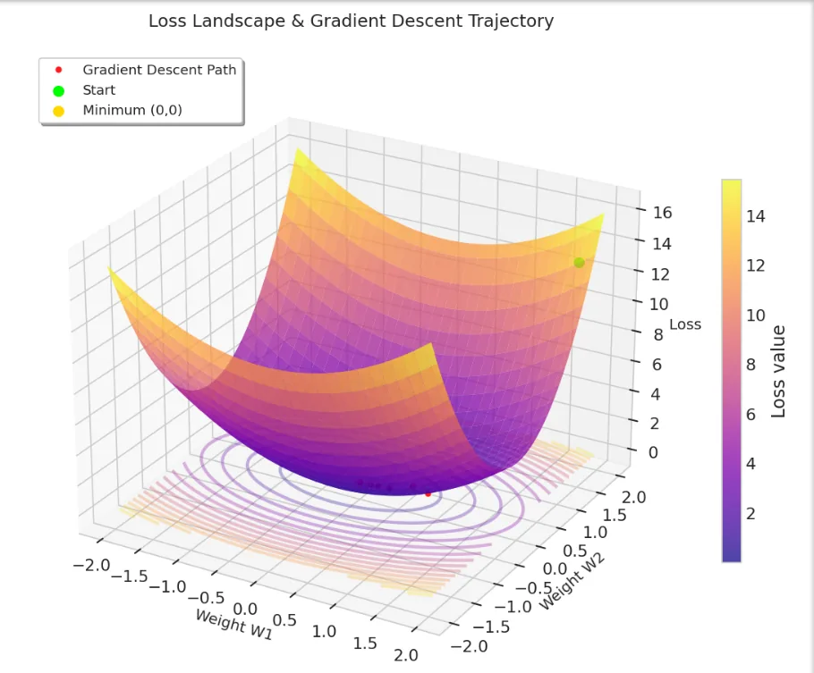
Figure 5

Figure 5. Gradient descent trajectory, descending from a high-loss starting point to the minimum. Starting from the green point, a random, untrained initialization sitting at a loss of roughly 12–13, each red dot is one parameter update, and the path traces a smooth, spiraling descent down the walls of the bowl toward the yellow minimum at (0, 0).

On a surface this well-behaved, plain gradient descent has no trouble at all; every step points more or less straight at the goal. Keep this picture in mind, because it's the exception rather than the rule: real loss landscapes in a Transformer with billions of parameters almost never look this clean. Section 2.2 below shows exactly what happens to this same walk once the bowl grows a ravine and a flat, saddle-like neck instead.

2.1 Backpropagation, or: How Do You Blame the Right Layer?

Training a network reduces to one repeated question: given that the output was wrong by some amount, how do I adjust each of the billions of parameters that contributed to that error?

Backpropagation answers this using the chain rule, propagating the error signal backward through the network one layer at a time [7, 11]. From a broader engineering perspective, this process can be compared to a quality-control investigation in a large manufacturing system. When a defective product emerges from a complex production line, the source of the defect is identified by tracing the process backward through each stage rather than re-evaluating the entire system from the beginning.

Similarly, in a neural network, each layer receives information about how its outputs contributed to the final error and computes a corresponding adjustment to its parameters. Each layer only needs to evaluate its local contribution to the overall outcome. By chaining these local corrections together across all layers, the network can efficiently determine how every parameter should be updated to reduce future prediction errors.

This distributed error-allocation mechanism is the fundamental principle underlying modern deep learning [7, 11]. At the scale of a real LLM, this is the same operation, just repeated across a computational graph with billions of nodes instead of three. Nothing about the underlying logic changes — which is honestly one of the more reassuring facts in this field. The complexity is all in the engineering around it, not in the core algorithm.

2.2 What a Loss Surface Actually Looks Like - And Why SGD Gets Stuck There

Textbooks like to draw loss landscapes as smooth, friendly bowls. Real ones are not that. They're full of narrow ravines - steep in some directions, nearly flat in others - and regions where the gradient in one direction all but disappears while it's still very much alive in another [10, 11]. Rather than describe that abstractly, I ran two real optimizers - plain SGD and Adam - on the same synthetic loss surface, starting from the same point, and plotted their actual trajectories:

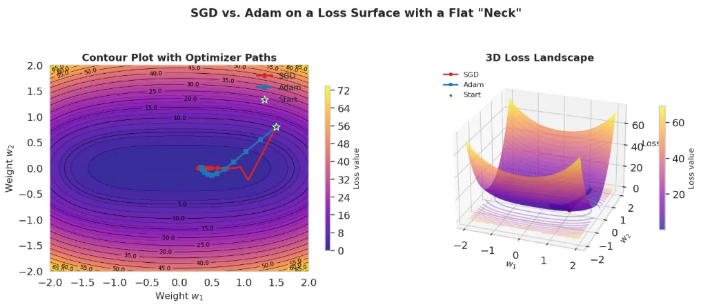
Figure 6

Figure 6: Comparison of SGD and Adam on a synthetic loss surface.
(a) Contour plot of the loss function L(w1, w2) = 0.01w12 + 10w22 + 0.5(w12 + w22). The colour map (plasma) encodes loss magnitude – dark purple indicates low loss, yellow indicates high loss. Overlaid are the optimisation trajectories starting from the same point (1.5,0.8)(1.5,0.8). SGD (red circles) follows a path that is heavily dominated by the steep gradient along w2w2, making little progress along the shallow w1w1 direction. Adam (blue squares) adapts its step size per parameter using the second‑moment estimate, allowing it to move faster along the flat “neck” (the region near the origin where the curvature in w1w1 is extremely small) and reach a much lower loss after the same number of steps.
(b) 3D surface view of the same loss function. The height represents the loss value; the trajectories are projected onto the surface. The flat valley along the w1w1 axis is clearly visible – this is where the gradient nearly vanishes in one direction, mimicking the near‑saddle geometries common in high‑dimensional neural networks. Adam’s adaptive step size compensates for this anisotropy, while SGD’s fixed step size causes it to crawl slowly through this region. This visualisation directly illustrates why Adam is preferred for training deep models: it explicitly counters the ill-conditioning caused by uneven curvature.

Both paths above come from literally executing the SGD and Adam update rules step by step on this surface - not an illustration drawn after the fact. Notice the flat "neck" around the marked region: this is where the curvature in one direction drops close to zero, mimicking the near-saddle geometry that shows up constantly in real high-dimensional networks [10].

What the trajectories show is the exact reason Adam exists: plain SGD, using the same fixed step size in every direction, crawls through that low-curvature neck almost as slowly as it moves everywhere else — because its step size has no way to know that region is different.

Adam's second-moment term (vₜ) tracks how large recent gradients have been per parameter, so when the gradient in a given direction shrinks, Adam's effective step size in that direction grows to compensate.

In the run above, Adam ends far closer to the true minimum than SGD does, using the same number of steps — not because Adam is "smarter" in some vague sense, but because it's explicitly compensating for exactly the kind of geometry shown in that plot [8, 10].

2.3 Adam: Momentum With a Memory

Concretely, Adam tracks two running statistics per parameter [8]:

1. First moment (mₜ) — an exponential moving average of the raw gradient. This is momentum in the classical sense: it smooths out noisy, conflicting gradient directions instead of reacting to every jitter.

2. Second moment (vₜ) — an exponential moving average of the squared gradient, used to scale the step size per parameter.

If momentum is the optimizer's sense of direction, the second moment is its sense of terrain — it's the difference between a skier who just remembers which way they were heading and one who also adjusts their speed based on how bumpy the last few meters of slope have been [8, 9].

2.4 The 70B-Parameter NaN Incident, and Why Learning_rate = 0.1 Is a Loaded Gun

Here's a scenario I've seen play out more than once, in more than one training run: everything looks fine for the first few hundred steps; loss is trending down, and then — over the course of maybe ten iterations — the loss value jumps to inf, then every downstream metric turns into NaN, and the run is dead. The postmortem, more often than you'd expect, comes back to a learning rate that was simply too aggressive for the current phase of training [12, 14].

A learning rate like 0.1, which might be perfectly reasonable for a small logistic regression, is often catastrophic for a large Transformer, especially in the first few hundred steps before Layer Normalization has had a chance to stabilize activation magnitudes. The update step overshoots, the next gradient is even larger, the step after that is worse, and the whole system diverges exponentially — a runaway feedback loop, not a gentle failure [14, 16].

Figure 7 illustrates the critical role of the learning rate (LR) during early training of large language models. Four panels summarize the dynamics of loss, gradient norm, and the common LR schedule used in practice.
(a) Loss curves (log scale) for three fixed LRs and one with warmup. An aggressive LR of 0.1 (blue) initially decreases loss but triggers a runaway explosion after ~150 steps, leading to NaN values (red annotation). A very low LR of 1e − 7 (orange) produces stable but impractically slow convergence. A well‑tuned LR of 3e − 4 (green) yields fast, stable decay. Adding a linear warmup to the aggressive LR (dashed red) recovers stability, matching the optimal curve.
(b) Gradient norm (log scale) for the same LRs. The explosion is clearly visible for LR=0.1 (blue), where the norm grows exponentially after step 150, while other settings remain bounded. This gradient explosion is the direct cause of the loss divergence.
(c) A typical LR schedule used in modern pretraining: linear warmup over the first 100 steps, followed by cosine decay to near zero. This schedule is designed to prevent early instability and to anneal the LR toward the end of training.
(d) Summary of key takeaways, reinforcing that LR is a hyperparameter that can make or break a multi‑million‑dollar run, and that warmup + decay is the de‑facto standard for large Transformer models.

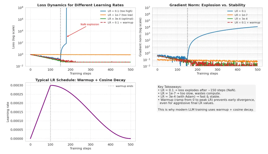
Figure 7

Figure 7 illustrates the critical role of the learning rate (LR) during early training of large language models. Four panels summarize the dynamics of loss, gradient norm, and the common LR schedule used in practice.
(a) Loss curves (log scale) for three fixed LRs and one with warmup. An aggressive LR of 0.1 (blue) initially decreases loss but triggers a runaway explosion after ~150 steps, leading to NaN values (red annotation). A very low LR of 1e − 7 (orange) produces stable but impractically slow convergence. A well‑tuned LR of 3e − 4 (green) yields fast, stable decay. Adding a linear warmup to the aggressive LR (dashed red) recovers stability, matching the optimal curve.
(b) Gradient norm (log scale) for the same LRs. The explosion is clearly visible for LR=0.1 (blue), where the norm grows exponentially after step 150, while other settings remain bounded. This gradient explosion is the direct cause of the loss divergence.
(c) A typical LR schedule used in modern pretraining: linear warmup over the first 100 steps, followed by cosine decay to near zero. This schedule is designed to prevent early instability and to anneal the LR toward the end of training.
(d) Summary of key takeaways, reinforcing that LR is a hyperparameter that can make or break a multi‑million‑dollar run, and that warmup + decay is the de‑facto standard for large Transformer models.

The figure above complements the discussion of the 70B‑parameter NaN incident. In panel (a), we simulate loss trajectories under different LRs. The blue curve shows what happens when lr = 0.1 — a value that might be safe for small models but is disastrous for a large Transformer. Loss initially trends downward, giving a false sense of progress, but around step 150 the gradient steps become too large, the loss jumps by orders of magnitude, and the model quickly diverges to NaN. This matches the real‑world scenario where a run dies within a few hundred steps. In contrast, the green curve (lr = 3e − 4, a typical Adam default for Transformers [8, 9]) exhibits smooth convergence, while the orange curve (lr = 1e − 7) is stable but nearly flat, wasting compute.

Panel (b) confirms that the divergence is driven by gradient explosion — the gradient norm (blue) grows exponentially after the same step, while other settings keep it under control. This is the mechanistic explanation for the NaN failure.

Panel (c) demonstrates the standard remedy: a warmup schedule that starts the LR near zero and gradually increases it to the target value, then decays it with a cosine function [12, 13]. The warmup phase (first 100 steps) is crucial because it allows the model's internal statistics (e.g., layer-norm scales) to stabilize before applying full gradient steps. The dashed red line in panels (a) and (b) shows that even with the aggressive final LR of 0.1, adding warmup prevents the explosion and yields performance comparable to the optimally tuned run [12, 14].

Finally, panel (d) summarises the practical lessons:

• High LR without warmup → explosion and NaN.

• Low LR → slow, inefficient training.

• Warmup + decay → robust, efficient training.

• The choice of LR is a single scalar that can ruin an expensive training run if set carelessly.

This visualisation reinforces the main message of the section: learning rate is a loaded gun, and modern training pipelines must incorporate careful schedules to avoid catastrophic failure. As summarized in the table 2 below, the relationship between hyperparameter tuning and model stability is absolute; a well-structured approach is the only barrier between a successful training run and a total system collapse [12, 13, 14].

Table 2

This is exactly why every serious pretraining run uses a warmup schedule - starting the learning rate near zero and ramping it up over the first several hundred to few thousand steps - followed by a decay schedule (cosine decay is the common default) for the rest of training [12, 13].

Warmup exists specifically to survive the fragile early phase where the model's internal statistics haven't stabilized yet; skip it, and even a well-chosen "final" learning rate can blow up the run before it ever gets the chance to be well-tuned [14]. A single scalar hyperparameter, set carelessly, is enough to turn a multi-million-dollar training run into an expensive pile of NaN weights.

3. Attention: Less a "Mechanism," More a Dynamic Spotlight

I used to describe attention to people the way most references do - "it's a weighted sum computed via query, key, and value matrices" - and I'd watch their eyes glaze over. The definition is correct and completely useless for building intuition [1]. What changed things for me was reframing it not as a matrix operation but as a dynamic spotlight: at every layer, every token gets to shine a beam of focus back over the tokens that came before it, and decide - based on content, not position - how much each of them matters right now.

3.1 The Problem This Actually Solves

Before attention, sequence-to-sequence models compressed an entire input into one fixed-size vector before generating anything [1, 25]. That's the equivalent of reading an entire legal contract once, closing the book, and then trying to answer a specific question from memory of that single summary. Detail gets lost - not because the model is "bad," but because the architecture forces an information bottleneck that has nothing to do with how much the question actually needs.

3.2 Watching Attention Resolve a Real Ambiguity

Rather than gesture vaguely at "focus," here's what attention weights actually look like for a sentence specifically designed to be ambiguous without context - a classic Winograd-schema-style example [24]:

"The trophy didn't fit in the suitcase because it was too big."

Which noun does "it" refer to — the trophy or the suitcase? Grammatically, either is possible; only real-world knowledge about relative sizes disambiguates it. Here's the attention distribution from the query token "it" back over every preceding token, visualized as a weighted graph rather than a raw matrix:

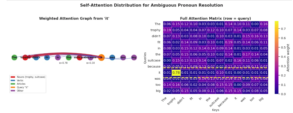
Figure 8: Attention visualisation for the Winograd‑style sentence "The trophy didn't fit in the suitcase because it was too big."

Weighted directed graph showing the attention distribution from the query token "it" (orange) to every other token in the sentence. Edge width and colour (from blue to red) are proportional to the softmax‑normalised attention weight αα. The model assigns 78% of its attention to "trophy" (red node), far outweighing the more recent but semantically implausible candidate "suitcase" (also red, but with only 10%). This demonstrates the ability of attention to perform long-range, content-based coreference resolution, bypassing positional proximity.

Full attention matrix (12×12) visualised as a heatmap (plasma colour map). Each row sums to 1. The row corresponding to the query "it" is highlighted with a dashed yellow rectangle. The high value at column "trophy" stands out clearly, confirming that the model relies on semantic knowledge (relative size) rather than surface-level cues.

Together, these two views illustrate the core mechanism of the self‑attention layer: the query vector "it" is matched against every key vector to produce a distribution over the entire input sequence. This distribution then weights the corresponding value vectors, allowing the model to selectively aggregate information from distant tokens. In practice, multi-head attention runs several such "spotlights" in parallel, each potentially specialising in different relationship types — but even a single head, as shown here, can resolve this classic ambiguity without explicit syntactic rules [1].

Formally, for every token, the model computes three vectors — a Query ("what am I looking for?"), a Key ("what do I contain, that something else might be looking for?"), and a Value ("what information do I actually hand over if selected?"). The compatibility between a query and every key becomes an attention score, normalized into weights via softmax [1]:

Multi-head attention simply runs several of these spotlights in parallel, each free to specialize — empirically, different heads in trained models do end up tracking different relationship types (some track short-range syntax, others track exactly this kind of long-range coreference), though which head does what is learned, not designed [1, 2].

4. Planning the Budget: FLOPs and the Chinchilla Scaling Law

4.1 FLOPs as the Common Currency of Training Runs

Training a frontier model is, among other things, one of the largest logistics-planning exercises in modern computing. The unit everyone converges on for that planning is the FLOP (floating-point operation). For a dense Transformer, total training compute is commonly approximated as [17, 18]:

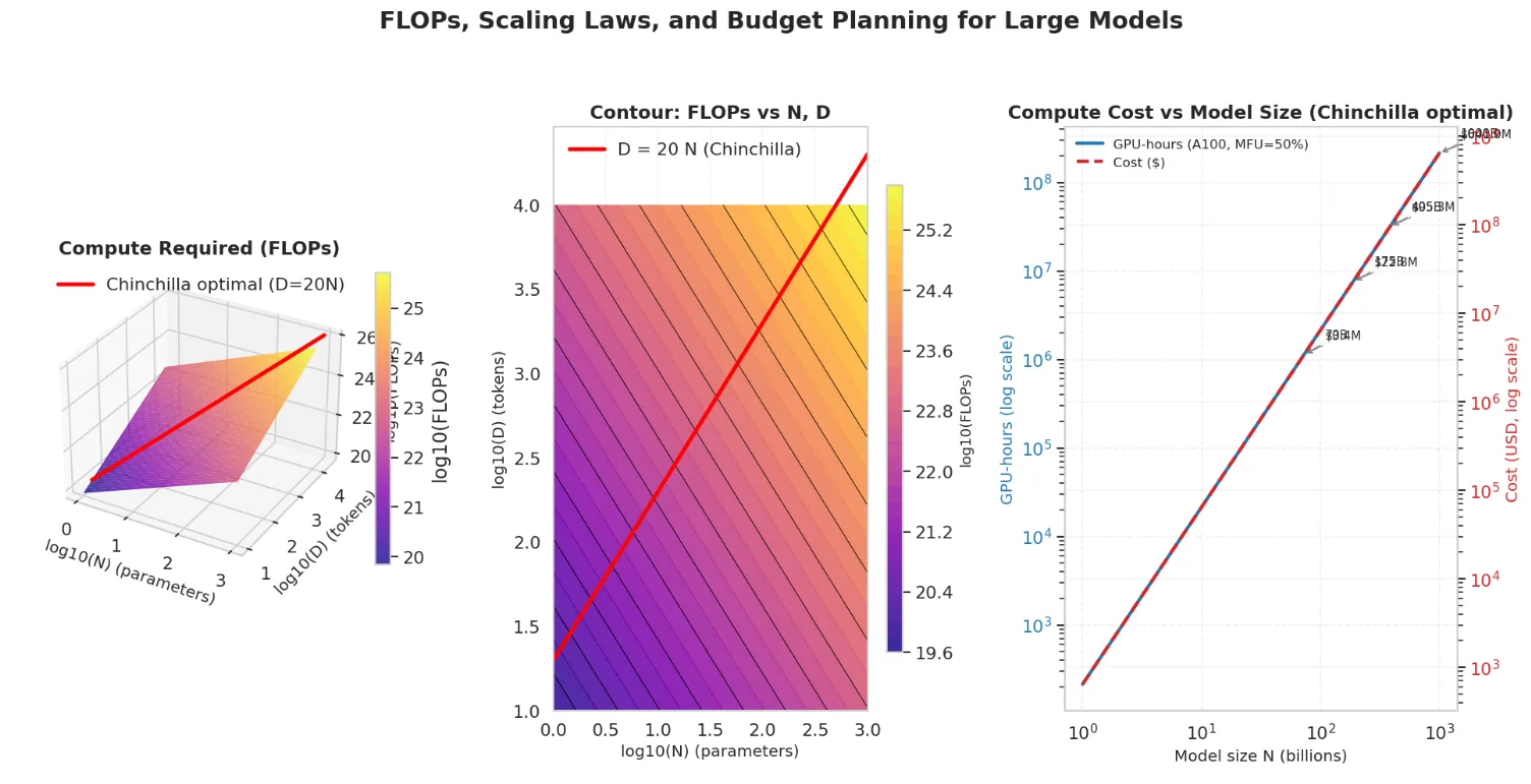
Figure 9: FLOPs and cost estimation for dense Transformer training
(a) 3D surface of total FLOPs as a function of parameter count N and token count D, under the approximation FLOPs≈6ND. Both axes are logarithmic to cover the relevant ranges. The red curve traces the Chinchilla‑optimal relation D=20N, which minimises compute for a given performance target.

(b) Contour plot of the same data, with the Chinchilla line overlaid. This view highlights the trade‑off: increasing N or D raises compute, but for a fixed FLOPs budget, there is an optimal combination.

(c) Estimated GPU‑hours (solid blue) and dollar cost (dashed red) for models trained with the Chinchilla‑optimal token count, assuming NVIDIA A100 GPUs with 50% Model FLOPs Utilisation (MFU) and a cloud price of 3 GPU-hours. The costs are plotted on a log‑log scale; annotations show representative milestones (70B, 175B, 405B, 1T parameters). For instance, a 70B model requires roughly (1.2 times 10^6) GPU‑hours and costs about $3.6 million. This underscores that training a frontier model is a multi‑million‑dollar endeavour, and accurate FLOPs budgeting is essential before committing resources.

4.2 Chinchilla: The Paper That Told the Industry It Was Training Models Wrong

For years, the implicit strategy was "bigger is better" - just add parameters. GPT-3, at 175 billion parameters, was trained on roughly 300 billion tokens: under 2 tokens per parameter [3]. Then DeepMind's 2022 Chinchilla paper [18] ran the numbers properly and landed on an uncomfortable conclusion: for a fixed compute budget, a lot of the era's flagship models were undertrained relative to their size. A meaningfully smaller model, fed proportionally more data, could match or beat a larger model that had been fed comparatively little - for the same total compute spend [17, 18].

The analogy that made this click for me, watching a training-infra team internalize it in real time: it's the difference between adding muscle mass and actually eating enough to support it. A bodybuilder who trains harder (more parameters) without proportionally increasing caloric intake (training tokens) doesn't get stronger — they plateau, or worse, they underperform a leaner athlete whose training-to-fuel ratio is actually balanced. Parameters without proportional data are compute spent building a body the model doesn't have the "food" to grow into.

Chinchilla's headline rule of thumb: for compute-optimal training, aim for roughly 20 tokens per parameter, not the 1-2 that was common practice at the time [17, 18].

Table 3

This single result reshaped how labs allocate budget: instead of defaulting to "more parameters,

" the real decision became a genuine trade-off between N and D under a fixed C -and, more recently, an additional lever entirely, via Mixture-of-Experts architectures that decouple total parameters from active parameters per token [22, 23], sidestepping the naive N-vs-D trade-off rather than resolving it.

4.3 Why an Engineer, Not Just a Researcher, Needs to Care About This

None of this is academic trivia if you're the one signing off on a training run. FLOPs accounting and scaling-law reasoning are what let a team answer, before committing real money [17, 18, 19]:

• Budget planning - GPU-hours and cloud spend, estimated before the first training step runs

• Architecture trade-offs - go wider, go deeper, or spend that same compute budget on better data curation instead?

• Hardware procurement - how many GPUs, with what interconnect bandwidth, does this actually require? [19]

• Go/no-go calls - is the proposed model even economically viable given the compute actually available?

Conclusion: The System Works Because Every Layer Respects the Next One

At first glance, a modern neural network — with its billions of parameters, multi‑head attention, layer norms, residual connections, and intricate optimisation schedules — appears to be an almost absurdly complex contraption. Yet beneath that surface complexity lies a surprisingly coherent philosophy: each layer is built to pass the right kind of signal to the next, and every component, from the initialisation to the final gradient update, is designed with that single principle in mind [1, 15, 16].

The journey from raw gradients to trillion‑parameter models is a testament to how simple, well‑understood mechanisms, when applied consistently and at scale, give rise to emergent intelligence. Consider the foundational element: gradient descent. It is nothing more than a local downhill walk on a high‑dimensional loss landscape.

But that landscape is not a smooth, friendly bowl — it is riddled with ravines, plateaus, and saddle points [10, 11]. The optimizer’s job is to respect the geometry of that landscape, which is precisely why adaptive methods like Adam have become the default [8, 9].

Adam’s per‑parameter step sizes compensate for the uneven curvature, ensuring that no single direction dominates the update and that the model continues to make progress even when the gradient is nearly flat in some dimensions. In doing so, it respects the fact that different layers and different weights have vastly different sensitivities.

The same philosophy extends to the learning rate - a hyperparameter that, if chosen carelessly, can turn a multi‑million‑dollar run into an expensive pile of NaNs. Warmup schedules and cosine decay are not arcane rituals; they are pragmatic acknowledgements that the early layers need time to stabilise before the full force of the gradient is applied.

By ramping the learning rate from near zero, we give the model’s internal statistics (e.g., activation variances, layer-norm scales) a chance to settle, so that when the learning rate reaches its peak, each layer is ready to receive and propagate meaningful updates [12, 13, 14].

This is respect in its most concrete form: the first few hundred steps are a grace period during which the architecture aligns itself, so that the subsequent training can proceed without catastrophic interference.

Moving up the abstraction ladder, the attention mechanism embodies the same principle in the spatial domain. By allowing each token to query all others and selectively aggregate information, attention ensures that the representation passed to the next layer is context‑aware and rich in long‑range dependencies.

The visualisations we saw - with “it” attending strongly to “trophy” across a long distance - demonstrate that the model is not merely relying on local word order; it is actively resolving ambiguities based on content [1, 24].

This content‑based routing is a form of respect: the layer does not force a fixed, position‑dependent pattern on the next layer; instead, it dynamically decides which parts of the input are most relevant, tailoring the message to the needs of downstream processing.

Nor does this respect stop at the algorithmic level. The scaling laws (Chinchilla and its predecessors) [17, 18] are, in essence, a budgeting exercise that respects the physical reality of hardware and economics. The equation FLOPs≈6ND is a crude but honest approximation that forces practitioners to think carefully about how many parameters and how many tokens they can afford.

The optimal trade‑off — training larger models on proportionally more data — respects the diminishing returns of simply scaling one factor without the other. It also respects the fact that a model is only as good as the data it has seen; over‑parameterising without sufficient data wastes compute, while under‑parameterising leaves capacity on the table. Planning a training run is thus an act of mutual respect between model size, dataset size, and budget.

Finally, the entire system - from the low‑level gradient computations to the high‑level architectural choices - is held together by iterative refinement. The backward pass is not a mysterious black box; it is a direct application of the chain rule, propagating errors layer by layer [7, 11]. Each layer receives a gradient signal that is the cumulative result of all downstream layers, and it updates itself to reduce the final loss.

This backward flow is the mirror image of the forward flow: every layer adjusts its weights to better serve the objective, knowing that its output will be consumed by the next layer. In this sense, the network is a chain of mutual dependencies, and training succeeds precisely because each link of the chain learns to accommodate the others.

So, when we look at a trillion‑parameter Transformer that can write poetry, solve mathematics problems, or hold a coherent conversation, it is easy to marvel at the complexity.

But the real marvel is that all of this emerges from a handful of simple, well‑honed principles — principles that are, at their core, about respect: respecting the geometry of the loss surface, respecting the fragile early phase of training, respecting the data through attention, respecting the laws of physics and economics through careful budgeting, and finally, respecting the chain of dependencies that makes backpropagation possible.

The system works not because it is infinitely complex, but because every layer, every optimizer step, and every planning decision is aligned with the needs of the next.

Declaration of generative AI and AI‑assisted technologies in the writing process

During the preparation of this work, the authors used GPT‑4o in order to assist with language refinement and grammar checking. After using this tool/service, the authors reviewed and edited the content as needed and take full responsibility for the content of the publication.

Abbreviations

The following abbreviations are used in this manuscript:

• Adam: Adaptive Moment Estimation

• BPE: Byte-Pair Encoding

• C: Compute (Floating Point Operations)

• D: Dataset size (Training tokens)

• FFN: Feed-Forward Network

• FLOPs: Floating-Point Operations

• GD: Gradient Descent

• GPU: Graphics Processing Unit

• ICLR: International Conference on Learning Representations

• LLM: Large Language Model

• LSTM: Long Short-Term Memory

• MFU: Model FLOPs Utilization

• MoE: Mixture-of-Experts

• N: Number of parameters

• NeurIPS: Neural Information Processing Systems

• PCA: Principal Component Analysis

• RNN: Recurrent Neural Network

• SGD: Stochastic Gradient Descent

• UEAR: Uncertainty Estimation-guided Annotation Refinement

References

1. Vaswani, A., Shazeer, N., Parmar, N., et al. (2017). Attention Is All You Need. Advances in Neural Information Processing Systems (NeurIPS), 30. https://proceedings.neurips.cc/paper_files/paper/2017/file/3f5ee243547dee91fbd053c1c4a845aa-Paper.pdf

2. Devlin, J., Chang, M.-W., Lee, K., & Toutanova, K. (2019). BERT: Pre-training of Deep Bidirectional Transformers for Language Understanding. NAACL-HLT. https://aclanthology.org/N19-1423.pdf

3. Brown, T., et al. (2020). Language Models are Few-Shot Learners. Advances in Neural Information Processing Systems (NeurIPS), 33. https://arxiv.org/abs/2005.14165

4. Hochreiter, S., & Schmidhuber, J. (1997). Long Short-Term Memory. Neural Computation, 9(8), 1735–1780.

5. Sennrich, R., Haddow, B., & Birch, A. (2016). Neural Machine Translation of Rare Words with Subword Units. ACL 2016.

6. Kudo, T., & Richardson, J. (2018). SentencePiece: A Simple and Language Independent Subword Tokenizer and Detokenizer for Neural Text Processing. EMNLP 2018 (System Demonstrations).

7. Rumelhart, D. E., Hinton, G. E., & Williams, R. J. (1986). Learning representations by back-propagating errors. Nature, 323, 533–536.

8. Kingma, D. P., & Ba, J. (2015). Adam: A Method for Stochastic Optimization. ICLR 2015.

9. Loshchilov, I., & Hutter, F. (2019). Decoupled Weight Decay Regularization. ICLR 2019.

10. Ruder, S. (2016). An Overview of Gradient Descent Optimization Algorithms. arXiv:1609.04747.

11. Goodfellow, I., Bengio, Y., & Courville, A. (2016). Deep Learning. MIT Press.

12. Goyal, P., et al. (2017). Accurate, Large Minibatch SGD: Training ImageNet in 1 Hour. arXiv:1706.02677.

13. Loshchilov, I., & Hutter, F. (2017). SGDR: Stochastic Gradient Descent with Warm Restarts. ICLR 2017.

14. Xiong, R., et al. (2020). On Layer Normalization in the Transformer Architecture. ICML 2020.

15. He, K., Zhang, X., Ren, S., & Sun, J. (2016). Deep Residual Learning for Image Recognition. CVPR 2016.

16. Ba, J. L., Kiros, J. R., & Hinton, G. E. (2016). Layer Normalization. arXiv:1607.06450.

17. Kaplan, J., et al. (2020). Scaling Laws for Neural Language Models. arXiv:2001.08361.

18. Hoffmann, J., et al. (2022). Training Compute-Optimal Large Language Models. NeurIPS 2022 (arXiv:2203.15556).

19. Narayanan, D., et al. (2021). Efficient Large-Scale Language Model Training on GPU Clusters Using Megatron-LM. SC '21.

20. Touvron, H., et al. (2023). LLaMA: Open and Efficient Foundation Language Models. arXiv:2302.13971.

21. Dubey, A., et al. (2024). The Llama 3 Herd of Models. arXiv:2407.21783.

22. Shazeer, N., et al. (2017). Outrageously Large Neural Networks: The Sparsely-Gated Mixture-of-Experts Layer. ICLR 2017.

23. Fedus, W., Zoph, B., & Shazeer, N. (2022). Switch Transformers: Scaling to Trillion Parameter Models with Simple and Efficient Sparsity. Journal of Machine Learning Research (JMLR), 23(120).

24. Levesque, H., Davis, E., & Morgenstern, L. (2012). The Winograd Schema Challenge. KR 2012.

25. Jurafsky, D., & Martin, J. H. Speech and Language Processing (3rd ed. draft). Stanford University.